Non-Linear ADP Controller¶

The below algorithms is given in the book Robust Adaptive Dynamic Programming.

Problem statements¶

Given the nonlinear system equation (2), design a control policy $u(t)$ that minimize the following cost function:

(1)¶ $V(x) = \int_0^\infty r(x(t),u(t))dt, \hspace{1cm} x(0)=x_0$

where $r(x,u)=q(x)+u^TR(x)u$ with $q(x)$ a positive definite function, and $R(x)$ is symmetric and positive definite for all $x \in \mathbb{R}^n$

If there exists a feedback control policy $u_0: \mathbb{R}^n \rightarrow \mathbb{R}^m$ that globally asymtotically stabilizes the system (2) at the origin and the associated cost as defined in (1) and there exists a continous differentiable function $V^*$ such that the Hamilton-Jacobi-Bellman (HJB) equation holds $H(V^*)=0$ then the control policy

(2)¶ $u^*(x) = -\frac{1}{2}R^{-1}(x)g^T(x)\nabla V^*(x)$

globally asymptotically stabilizes (2) at $x=0$ , and $u^*$ is also the optimal control policy

$V^*(x) = min_uV(x,u) \hspace{1cm} \forall x \in \mathbb{R}^n$

Off Policy Learning¶

Consider the system with the folowing control policy

(3)¶ $\dot{x} = f(x) + g(x)(u_0+e)$

where u0 is the initial admissible control policy and $e$ is the exploration noise then rewrite it as

(4)¶ $\dot{x} = f(x) + g(x)u_i(x) + g(x)v_i$

where $v_i = u_0-u_i+e$ .

Take the time derivative of $V_i(x)$ along (4) and integrate the result within interval $[t,t+T]$ to obtain:

(5)¶ $V_i(x(t+T)) - V_i(x(t)) = - \int_t^{t+T} [q(x)+u_i^TRu_i + 2u_{i+1}^TRv_i]d\tau$

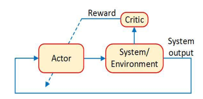
Because the formula (2) requires the knowledge of the dynamic of the system, it makes practical application limited. One may use neural networks to approximate the control policy $u_i$ (the actor)and the unknown cost function $V_i(x)$ (the critic).

$V_i(x) \approx \sum_{j=1}^{N_1}Wc_{i,j}\phi_j(x) \vspace{5mm} u_{i+1}(x) \approx \sum_{j=1}^{N_2}Wa_{i,j}\psi_j(x)$

where $\phi_j:\mathbb{R}^n \rightarrow \mathbb{R}$ and $\psi_j: \mathbb{R}^n \rightarrow \mathbb{R}^m$ are two sequences of linearly independent smooth basis function, $Wc, Wa$ is the weight of the neural networks.

Replacing them to the (5) and transform the result into the matrix, we have

(6)¶ $\begin{bmatrix} &\Delta\phi^T &-2(I_{u\psi}-I_{\psi\psi}(Wa_i^T \otimes I_\phi)) \end{bmatrix} \begin{bmatrix} &Wc_i^T \\ &vec(Wa_{i+1}^TR) \end{bmatrix} = \begin{bmatrix} I_q+I_{\psi\psi}vec(Wa_i^TRWa_i) \end{bmatrix}$

where $Wc_i = \begin{bmatrix} &Wc_{i,1}, &Wc_{i,2}, &..., &Wc_{i,N_2} \end{bmatrix}^T$ and the same for $Wa_i, \phi(x), \psi(x)$ and

$&\Delta\phi = \phi(x(t+T)) - \phi(x(t) \vspace{5mm} &I_q = \int_t^{t+T}q(x)d\tau \vspace{5mm} &I_{u\psi} = \int_t^{t+T}(u_0+e)^T\otimes \psi^Td\tau \vspace{5mm} &I_{\psi\psi} = \int_t^{t+T}(\psi^T\otimes \psi^T)d\tau \vspace{5mm} &I_\psi = np.eye(N_2)$

Finally, one can realize that the (6) is actually a fixpoint equation in the form

$A(w_i)C(w_{i+1}) = B(w_i)$

Note

the initial controller u0 must be admissible controller
the squences of basis functions $\phi_j(x), \psi_j(x)$ should be in the form of linearly independent smooth. Default basis functions is the polynomial functions, see OpenControl.ADP_control.NonLinController.default_psi_func() and OpenControl.ADP_control.NonLinController.default_phi_func()
the time interval T for data collection must be larger than the sample time
number of data $l >= n(n+1) + 2mn$
the default function $q(x)$ is $x^Tx$

Algorithm¶

Library Usage¶

Define a non-linear system like in System representation, then setup a simulation section by OpenControl.ADP_control.NonLinController.setPolicyParam() and perform simulation by OpenControl.ADP_control.NonLinController.offPolicy()

from OpenControl.ADP_control import NonLinController

##########define a controller##################
Ctrl = NonLinController(sys)
u0 = lambda x: 0      # the system is already globally stable
data_eval = 0.01; num_data = 80       # at leats n_phi+n_psi
explore_noise = lambda t: 0.2*np.sum(np.sin(np.array([1, 3, 7, 11, 13, 15])*t))

###############setup policy parameter############
Ctrl.setPolicyParam(data_eval=data_eval, num_data=num_data, explore_noise=explore_noise, u0=u0)
###############take simulation step##############
Wc, Wa = Ctrl.offPolicy()

then the optimal control policy is given by

uopt = lambda t,x: Wa.dot(Ctrl.psi_func(x))