Linear ADP Controller¶

The below algorithms is given in the book Robust Adaptive Dynamic Programming.

Problem statements¶

Given the linear system equation (1), design a linear quadratic regulator (LQR) in the form of $u=-Kx$ that minimizes the following cost function

$V(x) = \int_t^\infty (x^TQx+u^TRu)d\tau = x^TPx$

where $Q=Q^T \geq 0, R=R^T > 0$ .

The solution of this problem is $K*$ which is also the solution of the Riccati equation, can be obtained by OpenControl.ADP_control.LTIController.LQR(). However, this approach requires the knowledge of the system dynamic (the matrix A and B). The model-free approach below will resolve this problem.

Lets begin with another control policy $u=-K_kx+e$ where the time-varying signal e denotes an artificial noise, known as the exploration noise. Taking time derivative of the cost function and integrate it within interval $[t,t+\delta t]$ to obtain:

(1)¶ $x^T(t+\delta t) P_k x(t+\delta t) - x^T(t) P_k x(t) -2\int_t^{t+\delta t}e^T R K_{k+1} x d\tau = -\int_t^{t+\delta t}x^T Q_k x d\tau$

where $Q_k=Q+K_k^T R K_k$ .

We can see that this is the fix point equation, meaning that the K matrix can be solve by finite number of iteration. And because of no requirement of the system dynamic, it is a data-driven approach.

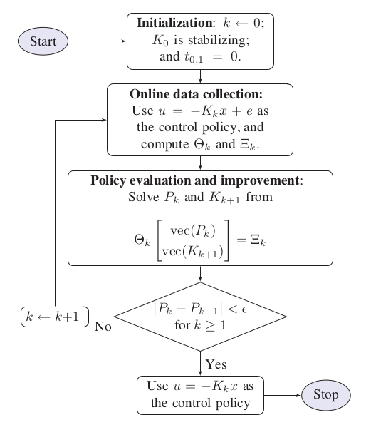
On-policy learning¶

For computational simplicity, we rewrite (1) in the following matrix form:

(2)¶ $\Theta_k \begin{bmatrix} vec(P_k) \\ vec(K_{k+1} \end{bmatrix} = \Xi_k$

where

$& \Theta_k = \begin{bmatrix} x^T \otimes x^T |_{t_{k,1}}^{t_{k,1+\delta t}} \hspace{1cm} -2\int_{t_{k,1}}^{t_{k,1+\delta t}}(x^T \otimes e^TR)dt x^T \otimes x^T |_{t_{k,2}}^{t_{k,2+\delta t}} \hspace{1cm} -2\int_{t_{k,2}}^{t_{k,2+\delta t}}(x^T \otimes e^TR)dt \vdots \hspace{1cm} \vdots x^T \otimes x^T |_{t_{k,l}}^{t_{k,l+\delta t}} \hspace{1cm} -2\int_{t_{k,l}}^{t_{k,l+\delta t}}(x^T \otimes e^TR)dt \\ \end{bmatrix}, \vspace{5mm} & \Xi_k = \begin{bmatrix} -\int_{t_{k,1}}^{t_{k,1+\delta t}}x^T Q_k x dt -\int_{t_{k,2}}^{t_{k,2+\delta t}}x^T Q_k x dt \vdots -\int_{t_{k,l}}^{t_{k,l+\delta t}}x^T Q_k x dt \end{bmatrix}$

Note

To adopt the persistent excitation condition, one must choose a sufficiently large number of data $l>0$ to satisfy the following condition:

$rank(\Theta_k) = \frac{n(n+1)}{2} + mn$

In practical, $l \geq n(n+1) + 2mn$
The time interval for each learning section is $l \cdot \delta t$ , so properly set OpenControl.ADP_control.LTIController.num_data and OpenControl.ADP_control.LTIController.data_eval to make sure the learning section not too slow

Algorithm¶

Library Usage¶

Setup a simulation section with OpenControl.ADP_control.LTIController and OpenControl.ADP_control.LTIController.setPolicyParam() then perform simulation by OpenControl.ADP_control.LTIController.onPolicy()

from OpenControl.ADP_control import LTIController

Ctrl = LTIController(sys)
# set parameters for policy
Q = np.eye(3); R = np.array([[1]]); K0 = np.zeros((1,3))
explore_noise=lambda t: 2*np.sin(10*t)
data_eval = 0.1; num_data = 10

Ctrl.setPolicyParam(K0=K0, Q=Q, R=R, data_eval=data_eval, num_data=num_data, explore_noise=explore_noise)
# take simulation and get the results
K, P = Ctrl.onPolicy()

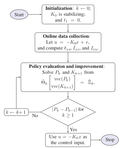
Off-policy learning¶

Let define some new matrices

$& \delta _{xx} = \begin{bmatrix} x\otimes x|_{t_1}^{t_1+\delta t}, & x\otimes x|_{t_2}^{t_2+\delta t}, & ..., & x\otimes x|_{t_l}^{t_l+\delta t} \end{bmatrix} ^T \vspace{5mm} &I_{xx} = \begin{bmatrix} \int_{t_1}^{t_1+\delta t}x\otimes xd\tau, & \int_{t_2}^{t_2+\delta t}x\otimes xd\tau, &..., & \int_{t_l}^{t_l+\delta t}x\otimes xd\tau \end{bmatrix} ^T \vspace{5mm} &I_{xu} = \begin{bmatrix} \int_{t_1}^{t_1+\delta t}x\otimes u_0d\tau, & \int_{t_2}^{t_2+\delta t}x\otimes u_0d\tau, &..., & \int_{t_l}^{t_l+\delta t}x\otimes u_0d\tau \end{bmatrix} ^T$

and $\Theta_k \in \mathbb{R}^{l\times (nn+mn)}, \Xi_k\in \mathbb{R}^l$ defined by:

$& \Theta_k = \begin{bmatrix} \delta_{xx}, & -2I_{xx}(I_n\otimes K_k^T R) - 2I_{xu}(I_n\otimes R) \end{bmatrix} \\ & \Xi_k = -I_{xx}vec(Q_k)$

then for any given stabilizing gain matrix $K_k$ , (1) implies the same matrix form as (2)

Algorithm¶

Library Usage¶

Setup a simulation section the same as the section then perform simulation by OpenControl.ADP_control.LTIController.offPolicy()

K, P = Ctrl.offPolicy()