Classic Control¶

About¶

module classiccontrol is the fundamental package needed for implementation control algorithms in with Python.

the main object of module is LTI system and relative algorithms, controller,… The Linear time-invariant system formulate in:

$\dot{x} = Ax + Bu \\ y = Cx + Du$

This package contains:

linearsystem.py: implement class LTI and basic attributes of system,
- system matrix
- dimension
- poles of system
- controllability and observability:
  
  Kalman standard
  
  Hatus standard
- simulation with controller and observer
bibo.py: implement algorithms for determining stability of LTI system
- Gerschgorin
- Lyapunov
- Hurwitz
controller.py: Design controller for LTI
- Pole statement:
  
  Roppernecker method
  
  Arckerman method
  
  Modal method
- Optimal control:
  
  LQR
observer.py: Design observer for LTI
- Luenberger observer
utils.py: collection of small and common Python functions which re-use a lots in difference package

This manual contains many examples of use, usually prefixed with the Python prompt >>> (which is not a part of the example code). The examples assume that you have first entered:

from OpenControl import classiccontrol

Declare LTI system:

import numpy as np

A = np.array([[0,          1,    0,     0],
              [28.0286,    0,    0,     0],
              [0,          0,    0,     1],
              [-1.4014,    0,    0,     0]])

B = np.array([[    0     ],
                -1.5873  ],
                   0     ],
                 0.6349  ]])

C = np.array([[1,    0,    0,     0],
              [0,    1,    0,     0],
              [0,    0,    1,     0],
              [0,    0,    0,     1]])

sys = classiccontrol.linearsystem.LTI(A=A, B=B, C=C)

Controllability and observability¶

Kalman standard:

Theorem: The linear continuous-time system is controllable if and only if the controllability matrix has full rank.

The observability matrix, in this case, defined by:

Theorem: The linear continuous-time system is controllable if and only if the controllability matrix has full rank.

The controllability matrix, in this case, defined by:

Hatus standard:

System is controllable if matrix: is full rank with any s.

$Rank(sI - A, B) = n System is observable if matrix: is full rank$

Stability¶

Gerschgorin:: A is system matrix. Elements of A, aij.

$Ri(A) = \sum_{j=1, j\neq i}|a_{ij}$

Hurwitz:

system is stable if all the eigen values of system matrix on the left of complex coordinate

Lyapunov:

A is hurwitz, If there exist a positive definite squad matrix $Q=Q^T$ such that $P=-(QA + A^TQ)$ is a positive definite matrix

b) A is hurwitz ,If there exist a positive definite squad matrix $P=P^T$ such that equation $P=-(QA + A^TQ)$ got a solution $Q$ and Q is positive definite squad matrix

Stability of system:

#select the algorithms

sys.is_stable(algorimth='gerschgorin')
sys.is_stable(algorimth='hurwitz')
sys.is_stable(algorimth='lyapunov')

Code examples 1¶

This experiment from the paper ‘Observer-Based Controllers for Two-Wheeled Inverted Robots with Unknown Input Disturbance and Model Uncertainty’ Declare LTI system:

import numpy as np

A = np.array([[0,          1,    0,     0],
              [28.0286,    0,    0,     0],
              [0,          0,    0,     1],
              [-1.4014,    0,    0,     0]])

B = np.array([[    0     ],
                -1.5873  ],
                   0     ],
                 0.6349  ]])

C = np.array([[1,    0,    0,     0],
              [0,    1,    0,     0],
              [0,    0,    1,     0],
              [0,    0,    0,     1]])

sys = classiccontrol.linearsystem.LTI(A=A, B=B, C=C)

Basic attribute of LTI system.

stability = sys.is_stable()
controllability =sys.controllable()
observability = sys.observable()
poles = sys.eigvals()

simulate Open-loop system.

sys.setup_simulink(max_step=1e-3, algo='RK45', t_sim=(0,10), x0=None, sample_time = 1e-2,z0=None)
time_array,state,output = sys.step_response()

Design controller

controller = classiccontrol.controller.PoleStatement(pole=[-3,-4,-5,-6], system=sys)
R = controller.compute()

Design observer

observer = classiccontrol.observer.Luenberger(pole=[-3,-4,-5,-6], system=sys)
L = observer.compute()

simulate Closed-loop system with state-feedback controller R

sys.setup_simulink()
time_array,state,output,state_obs = sys.apply_state_feedback(R)

simulate Closed-loop system with output-feedback L-R

sys.setup_simulink()
time_array,state,output,state_obs = sys.apply_output_feedback(L,R)

Code examples 2¶

simulate a Two-Wheeled Inverted Rotbots. cited in the paper ‘Observer-Based Controllers for Two-Wheeled Inverted Robots with Unknown Input Disturbance and Model Uncertainty’

object got the folowing parameters:

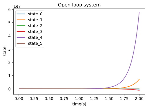
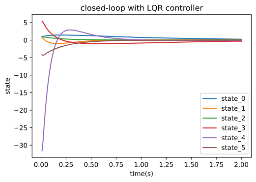
Simulate behavior of open-loop system Design LQR controller Simulate behavior of closed-loop system with LQR controller

import numpy as np
from OpenControl import classiccontrol
A = np.array([0,0,0,1,0,0,0,0,0,0,1,0,0,0,0,
        0,0,1,0,-14.5,0,-32.47,1.07,0,0,162.07,
        0,242.88,-8.01,0,0,0,0,0,0,-5.66]).reshape(6,6)
B = np.array([0,0,0,0,0,0,107.159,107.159,-801.536,
        -801.536,-191.648,191.648]).reshape(6,2)
C = np.eye(6)
Q = np.diag([4,3,20,3.5,0.001,0.9])
R = np.diag([1,1])
sys = classiccontrol.linearsystem.LTI(A=A,B=B,C=C)
ctl = classiccontrol.controller.LQR(sys,Q,R)
R = ctl.compute()
sys.setup_simulink(t_sim=(0,2))
time_array, state,output = sys.step_response()
time_array2, state2,output2 = sys.apply_state_feedback(R)

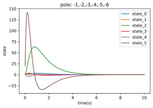
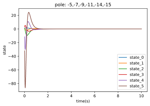
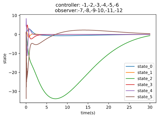
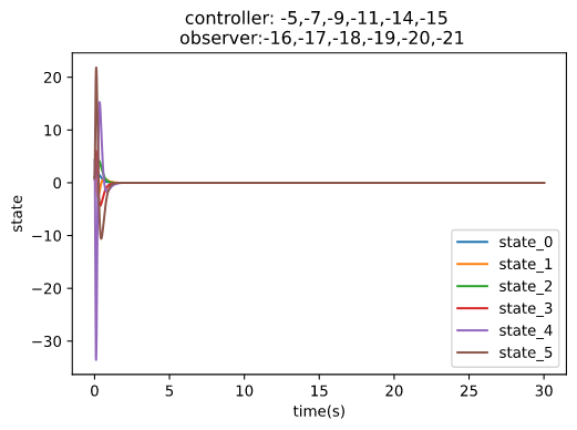
Design and simulate pole-statement controller 1 with pre-define poles : -1,-2,-3,-4,-5,-6 Design and simulate pole-statement controller 2 with pre-define poles : -5,-7,-9,-11,-14,-15 Design Luenberger observer with pre-define poles : -7,-8,-9,-10,-11,-12 Design Luenberger observer with pre-define poles : -16,-17,-18,-19,-20,-21

ctl_1 = classiccontrol.controller.PoleStatement(pole=[-1,-2,-3,-4,-5,-6],system=sys)
R1 =ctl_1.compute()
obs_1 = classiccontrol.observer.Luenberger(pole=[-7,-8,-9,-10,-11,-12],system=sys)
L1 = obs_1.compute()
ctl_2 = classiccontrol.controller.PoleStatement(pole=[-5,-7,-9,-11,-14,-15],system=sys)
R2 =ctl_2.compute()
obs_2 = classiccontrol.observer.Luenberger(pole=[-16,-17,-18,-19,-20,-21],system=sys)
L2 = obs_2.compute()
sys.setup_simulink(t_sim=(0,50))#,x0=np.random.randint(-1,1,(6,1)))
time_array1, state1,output1 = sys.apply_output_feedback(L1,R1)
time_array2, state2,output2 = sys.apply_output_feedback(L1,R1)
time_array3, state3,output3,z0 = sys.apply_output_feedback(L1,R1)
time_array4, state4,output4,z1 = sys.apply_output_feedback(L2,R2)